Gradient descent, Newton-like
February 5, 2019 — January 15, 2024
Suspiciously similar content
NB ⚠️⛔️☣️: Under reconstruction; I think I need to characterise the 2nd-order Hessian approximations better.
Newton-type optimization, unlike basic gradient descent, uses (possibly approximate) 2nd-order gradient information to find the argument which minimises \[ x^*=\operatorname{arg min}_{\mathbf{x}} f(x) \] for some objective function \(f:\mathbb{R}^n\to\mathbb{R}\).
Optimization over arbitrary functions typically gets discussed in terms of line-search and trust-region methods, both of which can be construed, AFAICT, as second order methods. Although I don’t know of a first order trust region method; what would that even be? I think I don’t need to care about the distinction for the current purpose. We’ll see.
Can one do higher-than-2nd order optimisation? Of course. In practice, 2nd order is usually fast enough and has enough complications to keep one busy, so the greater complexity and per-iteration convergence rate of a 3rd order method does not usually offer an attractive trade-off.
Here are some scattered notes which make no claim to comprehensiveness, comprehensibility or coherence.
1 General
Robert Grosse, Second-Order Optimization is a beautiful introduction as part of CSC2541 Topics in Machine Learning: Neural Net Training Dynamics. There is a whole series (Grosse 2021a, 2021b, 2021c) of IMO beautifully written lectures on this.
2 One-dimensional Newton
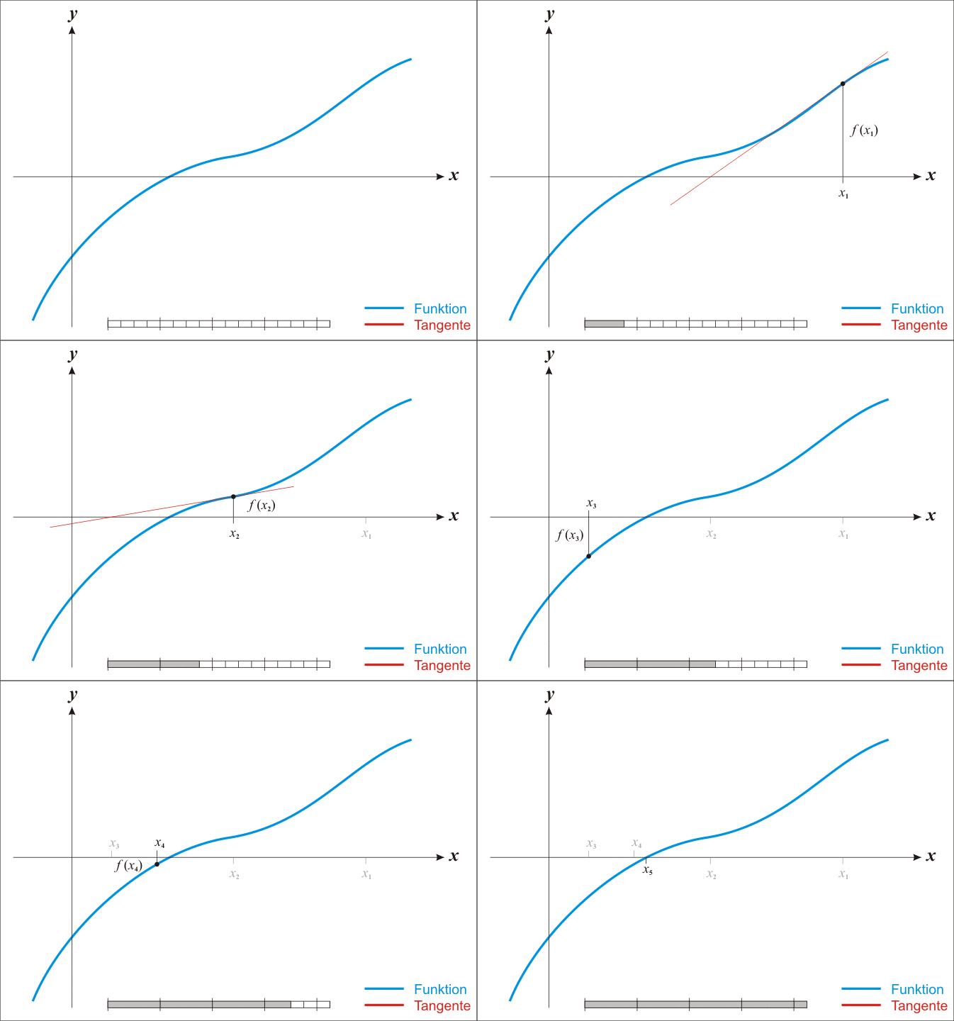
The basic case is simple; we get into difficulties with the multidimensional stuff in a moment. From school one might remember that classic so-called Newton method for iteratively improving a guessed location \(x_{k}\) for a root of a 1-dimensional function \(g:\mathbb{R}\to\mathbb{R}\):
\[ x_{k+1}=x_{k}-\frac{g\left(x_{k}\right)}{g'\left(x_{k}\right)} \]
Under the assumption that it is twice continuously differentiable, we can find stationary points—zeros of the derivative—of a function \(f:\mathbb{R}\to\mathbb{R}\). (i.e. extrema and saddle points, which might in fact be minima.) \[ x_{k+1}=x_{k}-\frac{f'\left(x_{k}\right)}{f''\left(x_{k}\right)} \]
How and why does this work again? Loosely, the argument is that we can use the Taylor expansion of a function to produce a locally quadratic model for the function, which might be not at all globally quadratic.
3 Multidimensional Newton
Returning to the objective with a multidimensional argument \(f:\mathbb{R}^n\to\mathbb{R},\) Taylor’s theorem for twice continuously differentiable functions tells us that \[\begin{aligned} f(x+p)&= f(x)+\nabla^{\top} f (x+p)p +\frac{1}{2}p^{\top} \nabla^2f(x+p)p + p^{\top}R(x+p)p\\ \end{aligned}\] and \(\lim _{p \rightarrow 0} R(x+p)=0\).
Putting the remainder in Cauchy form, this tells us \[ f(x+p)=f(x)+\nabla f^{\top}(x)p+\frac{1}{2}p^{\top}\nabla^2f(x+tp)p \] for some \(t\in(0,1)\).
Generally, we might take a local quadratic model for \(f\) at \(x+p\) as \[ \nabla f(x+p)\simeq m_x(p)= f(x)+\nabla f^{\top}(x)p+\frac{1}{2}p^{\top}\nabla^2f(x)p \] for some \(t\in(0,1)\).
If we ignore some subtleties and imagined this quadratic model was true, it would have an extremum where the directional derivative of this model vanished, i.e. $ m_x(p)$ where \(\nabla m_x(p):=\nabla f(x)+\nabla^2 f(x)p\). This would be satisfied at \[\begin{aligned} \nabla f(x)+\nabla^2 f(x)p &= 0\\ \nabla f(x)&=-\nabla^2 f(x)p\\ p&=-[\nabla^2 f(x)]^{-1}\nabla f(x)\\ \end{aligned}\]
From this we get the multidimensional Newton update rule, by choosing for each \(x_{k}\) the locally optimal \(p\) quadratic approximation: \[ x_{k+1}= x_{k}-\left[ \nabla^2 f\left( x_{k}\right)\right]^{-1} \nabla f\left( x_{k}\right), n \geq 0 \]
In practice the quadratic model is not true (or we would be done in one step) and we would choose a more robust method that by using a trust region or line-search algorithm to handle the divergence between the model and its quadratic approximation. Either way the quadratic approximation would be used, which would mean that the inverse Hessian matrix \(\left[ \nabla^2 f\left( x_{k}\right)\right]^{-1}\) would be important.
🏗 Unconstrained assumption, need for saddle points not just extrema with Lagrange methods, positive-definiteness etc.
4 Gauss-Newton
A reasonably clear Stackeschange answer that will do for now: Difference between Newton’s method and Gauss-Newton method.
5 Generalized Gauss-Newton
NB ⚠️⛔️☣️: This sections is vague half-arsed notes of dubious accuracy.
The generalized Gauss-Newton approximation (GGN) (Martens and Grosse 2015). replaces an expensive second order derivative by a product of first order derivatives. Used in (Foong et al. 2019; Immer, Korzepa, and Bauer 2021).
6 Fisher method
I haven’t actually worked out what this is yet, nor whether it relates or is filed correctly there. But I think that it is natural gradient descent.
7 Quasi Newton methods
Secant conditions and approximations to the Hessian. Let’s say we are designing a second-order update method. See e.g. Nocedal and Wright (2006).
In BFGS the approximate Hessian \(B_k\) is used in place of the true Hessian.
Given the displacement \(s_{k}\) and the change of gradients \(y_{k}\), the secant equation requires that the symmetric positive definite matrix \(B_{k+1}\) map \(s_{k}\) into \(y_{k}.\)
\[ H_k(x^{(k)} − x^{(k−1)}) = \nabla f(x^{(k)}) − \nabla f(x^{(k−1)}) \]
… We hope to get from this the secant condition.
\[ B_{k+1} s_{k}=y_{k} \]
TODO: compare and contrast to the Wolfe conditions on step length.
🏗
8 Hessian free
Second order optimisation that does not require the Hessian matrix to be given explicitly. I should work out the boundaries of this definition. Does it include Quasi Newton? CGD? Intersect with? Overlap? 🏗
Andre Gibiansky wrote an example for coders.
9 Stochastic
See stochastic 2nd order gradient descent for some bonus complications.

