Gaussian Ensemble Belief Propagation
A method which improves our ability to solve important tricky problems, such as whether your house will flood tomorrow based on what the satellite says today
April 15, 2024 — February 6, 2025
Suspiciously similar content
Assumed audience:
Interested laypeople, working statisticians, maybe ML people?
We recently released a paper on a method called GEnBP (MacKinlay et al. 2025). GEnBP was an unexpected discovery: we were working on exotic methods for solving some important complicated geospatial problems (see below) and discovered an unusual but simple method that ended up outperforming our complex initial approach and existing solutions.
This is useful not just because we like being the best. 😉 Geospatial problems are crucial for our future on this planet. Many people, even inside the worlds of statistics, may not realise the difficulties of solving such problems. I’m excited about our findings for many reasons. Here I’ll explain both the difficulties and our solution.
1 The problems we want to solve
In statistical terms, our target problems are
- high-dimensional
- noisy
- defined by complicated physics models
- hierarchical (in the technical sense that “things influence each other”) and
- at massive scale.
An example of why we care about such problems is that they pop up naturally in modern science, e.g. Figure 2. That diagram is a simplified representation of what scientists want to do when trying to use lots of different kinds of data to understand something big, in the form of a graphical model. In this case, it is a graphical model of the ocean and the atmosphere, the kind of thing we need to do when we are modelling the planetary climate. An arrow \(X \rightarrow Y\) means (more or less) “\(X\) causes \(Y\)” or “\(X\) influences \(Y\)”. We can read off the diagram things like “The state of the ocean on day 3 influences the state of the ocean on day 4 and also the state of the atmosphere on day 4.” Also, we have some information about the state of the ocean on that day because it is recorded in a satellite photo, and some information about the atmosphere that same day from radar observations.

Now the question is: how can we put all this information together? If I know some stuff about the ocean on day 3, how much do I know about it on day 4? How much can I use my satellite images to update my information about the ocean? How much does that satellite photo actually tell me?
What we really want to do is exploit our knowledge of the physics of the system. Oceans are made of water, and we know a lot about water. I would go so far as to say we are pretty good at simulating water. For a neat demonstration of fluid simulation, see Figure 3, showcasing work from our colleagues in Munich. You could run this on your home computer right now if you wanted.

The problem is that when these simulators have all the information about the world, they are not bad at simulating it. But in practice, we don’t know everything there is to know. The world is big and complicated, and we are almost always missing some information. Maybe our satellite photos are blurry, don’t have enough pixels, or a cloud wandered in front of the camera at the wrong moment, or any one of a thousand other things.
Our goal in the paper is to leverage good simulators to get high-fidelity understanding of complicated stuff even when we have partial, noisy information. There are a lot of problems we want to solve at once here: We want to balance statistical and computational difficulty, and we want to build on the hard work of scientists who came before us.
There is no silver bullet method that can solve this for every possible system; everything has trade-offs; we will need to make the best guess we can given how much computer time we have.
We care about problems like this because basically anything at scale involves this kind of issue. Power grids! Agriculture! Floods! Climate! Weather! Most things that impact the well-being of millions of people at once end up looking like this. All of these important problems are difficult to get accurate results for because it is hard to make efficient use of our data, which is incredible but doesn’t tell us exactly what we truly want.
We think that in GEnBP, we have good methods solving this punishing problem.
2 Our solution
Our approach utilises existing simulators, originally designed for full information, to make educated guesses about what is going on by feeding in random noise to indicate our uncertainty. We check the outputs of these educated guesses (the prior for statisticians following along at home). Then we make an update rule that uses the information we have to improve these guesses until we have squeezed all the information we can out of the observations.
How exactly we do this is not complicated, but it is technical. Long story short: our method is in a family called belief propagation methods, which tells us how to update our guesses when new information arrives. Moreover, this family updates our guesses using only local information — for example, we only look at “yesterday” and “today” together rather than looking at all the days at once, which is too much information to look at for each step. Instead, we walk through all the data, bit-by-bit. Each time we try to squeeze more information out of the update, until we have something like a best guess. In fact the “best” guess ends up being useless; What we end up with is a family of guesses, each of which is a little bit different, and we can use these to work out how certain we are about our final answer. Collectively those guesses end up being a good approximation to the true answer.

The minimum viable example for us, and the one we tackle first in the paper, is a (relatively) simple test case, Figure 4. This is what’s known as a system identification problem. Each circle represents a variable (i.e. some quantity we want to measure, like the state of the ocean), and each arrow signifies a ‘physical process we can simulate’. The goal is to identify the query parameter (red circle) from the evidence, i.e. some noisy observations we made of the system.
The data in this case come from a fluid simulator, modelling a fluid flowing around a doughnut-shaped container. We didn’t collect actual data for this experiment, which is just as well — I’m a computer scientist, not a lab scientist 😉. Our observations are low-resolution, distorted, and noisy snapshots of the state of the fluid. The red circle indicates a hidden influence on the system; in our case, it is a force that “stirs” the fluid. Our goal is “can I work out what force is being applied to this fluid by taking a series of photos of it?”
In fact, many modern methods ignore this hidden influence entirely; the Ensemble Kalman Filter, for example, struggles with hidden influences. But in practice, we care a lot about such hidden influences. For one thing, such hidden factors might be interesting in themselves. Sailors, for example, care not just about the ocean waves, but also about what the waves’ behaviour might indicate about underwater hazards. Also, we want to be able to distinguish between external influences and the dynamics of a system itself, because, for example, we might want to work out how to influence the system. If I am careful about identifying which behaviour comes from some external factor, this lets me deduce what external pressure I need to apply to it myself. What if I want to not only work out how the water flows but how it will flow when I pump more water in?
This challenge belongs to a broader field known as Causal inference from observational data, which concerns itself with unravelling such complexities. I feel that is probably worth a blog post on its own, but for now let us summarise it with the idea that a lot of us think it is important to learn what is actually going on underneath, rather than what only appears to be going on.
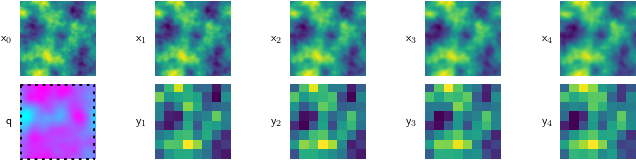
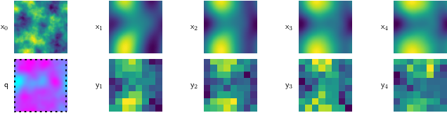
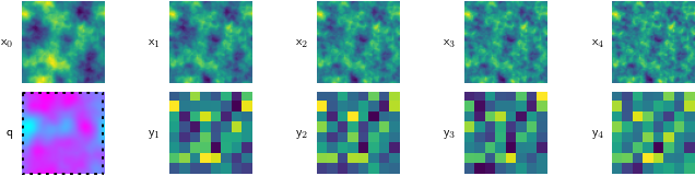
Because this is a simulated problem, we can cheaply test our method against many different kinds of fluids. So, we do, testing our method on runny fluid Figure 5 (a), thick, viscous fluid Figure 5 (c), and stuff in between Figure 5 (b).
For all of these, the starting condition (\(\mathsf{x}_0\)) is the same, and our goal is to find the magenta-tinted answer (\(\mathsf{q}\)).
3 Performance
Having outlined the problem, let’s now unpack the performance of GEnBP, our proposed solution. How good is GEnBP, relatively speaking? As far as we can tell, there is only one real competitor in this space, which is classic Gaussian Belief Propagation (GaBP). More on GaBP below. We use that as a baseline.
It’s challenging to present multiple simulations from a 2D fluid simulator effectively, as they primarily consist of colourful squares that are not immediately interpretable. This is easier if we can plot it in one spatial dimension. For demonstration purposes, I set up a special 1D pseudo-fluid simulator. The question in this one is, “How well do our guesses about the influencing variable converge on the truth?”
The classic GaBP results Figure 6 are… OK, I guess? In the figure, the red lines represent our initial educated guesses (‘prior’), and the blue lines show the optimised final guesses (‘posterior’), compared to the dotted black line representing the truth. The blue guesses are much better than the red ones, for sure, but they are not amazing. Our fancy GEnBP guesses Figure 7 are way better, clustering much closer to the truth. So tl;dr on this (admittedly made-up) problem, our method does way better at guessing the ‘hidden influence’ on the system.


This example is extremely contrived though! So, let us quantify how much better the answers are on the more complex, more realistic 2-dimensional problem.
At this stage, our approach manages millions of pixels, surpassing the capabilities of classical methods. GaBP tends to choke on a few thousand pixels. But our method can eat up big problems like that for breakfast.

What we are looking at in this graph are some measures of performance as we scale up the size of the problem, i.e. the number of pixels. The top graph displays the execution time, which ideally should be low, plotted against the problem size, measured in pixels. Notice that as the problem gets bigger, GaBP gets MUCH slower.
For the curious, it scales roughly cubically, i.e. \(\mathcal{O}(D^3)\). GaBP is generally much slower for the kind of problems we care about. Moreover, eventually, GaBP runs out of memory. The middle graph shows something else interesting: GEnBP also has superior accuracy to the classic GaBP, in the sense that its guesses are on average closer to the truth. The bottom graph shows the posterior likelihood, which essentially tells us how confident our method is in the vicinity of the truth.
We have been strategic with our choice of problem here: GaBP is not amazing at fluid dynamics precisely like this, and that is kind of why we bother with this whole thing. GaBP has trouble with very nonlinear problems, which are generally just hard. GEnBP has some trouble with them too, but often much less trouble.

In Figure 11, we test both these methods on a lot of different fluid types and see how they go. GEnBP is best at speed for… all of them. The story about accuracy is a little more complicated. We win some, and we lose some. So, it’s not a silver bullet.
However, GEnBP can tackle problems far beyond GaBP’s capacity, and it often has superior accuracy even in scenarios manageable by GaBP.
4 How it works
The core insight of our work is combining the best elements of the Ensemble Kalman Filter (EnKF) and classic Gaussian belief propagation (GaBP). We’ve developed an alternative Gaussian belief propagation method that outperforms the classic GaBP. These methods are closely related, and yet their research communities don’t seem to be closely connected. GaBP is associated with the robotics community. If you have a robotic vacuum cleaner, it probably runs on something like that. Rumour holds that the Google Street View software that makes all those Street View maps uses this algorithm. There are many great academic papers on it (e.g. Bickson 2009; Davison and Ortiz 2019; Murphy, Weiss, and Jordan 1999; Ortiz, Evans, and Davison 2021; Dellaert and Kaess 2017).
The Ensemble Kalman Filter is widely used in areas such as weather prediction and space telemetry. While I don’t have visually striking demos to share, I recommend Jeff Anderson’s lecture for a technical overview. Here are some neat introductory papers on that theme: (Evensen 2009a, 2009b; Fearnhead and Künsch 2018; Houtekamer and Zhang 2016; Katzfuss, Stroud, and Wikle 2016).
As far as work connecting those two fields, there does not seem to be much, even though they have a lot in common, which is surprising. That is where our GEnBP comes in. Our method is surprisingly simple, but it appears to be new, at least for some value of new.
Connecting the two methods is mostly a lot of “manual labour”. We use some cool tricks such as the Matheron update (Doucet 2010; Wilson et al. 2020, 2021), and a whole lot of linear algebra tricks such as Woodbury identities. Details in the paper.
5 Advanced problem: reality gap
So far, we have done fairly “normal” things with this algorithm, which feels like a waste to me. Let’s get weird.
The example above is system identification. We can target the more challenging, arbitrarily complicated, data-assimilation-type problem that doesn’t have all the shortcuts that researchers use in system identification problem; remember the big game we talked about in Figure 4?
It turns out that we can actually solve these too. Figure 10 graphs an emulation problem, which is a little complicated to explain and also generally regarded as extremely challenging-to-impossible.
Our task here is to once again approximate that fluid simulation, but in a more difficult and also more realistic setting like the ones we encounter in the real world.
Imagine this: I want to simulate the weather’s behaviour on the planet. I have high-quality simulators, which are too expensive to run all the time. I have noisy and imperfect observations from some satellite, which are pretty cheap.1 This kind of noisiness is the standard in weather forecasting, it turns out. When you think about it, the weather satellites can show us moving clouds and such, but as far as the actual air itself goes, clearly there is a lot of guesswork about what that giant volume of air molecules is actually doing. Is it hot? Cold? Moving? Which way? How about that bit of air just above the first bit? This is the kind of stuff that simulators are good at, but it is painful trying to run them “in reverse” and work out what inputs to the simulator would produce those satellite images we can actually observe.
We would like it if we could train a neural network to approximate the simulator, so that I could run the neural network instead of the simulator. Neural networks are much nicer in all kinds of ways, and much easier to work with than full simulators. But also they are kind of “fake”; an approximation to a simulation of reality is too many steps removed from reality to be trustworthy. Can we ensure that our nice tractable neural nets are actually a good approximation to the real world? This is called a ‘reality gap’ problem in my organisation.
It turns out GEnBP can do this; we can set up the problem of “turn my emulator for idealised weather into an emulator for real weather” as a graphical model, and then solve it with GEnBP.
The trick is we train a Bayesian neural network, which is a neural network that outputs a probability distribution instead of a single vector. By using a Fourier Neural Operator, we can even make that ‘emulator’ network compact (about \(10^6\) weights). We train that on the high-quality simulator, so it’s a high-fidelity approximation of the simulator.
Now, this emulator is going to be a pretty rough match to reality because it is trained on the simulator, not the real world. BUT! The noisy observations of the real world relate to this emulator via another graphical model and use that to update the neural network to be a better approximation of the real world. The whole setup looks like Figure 10.


Now I’m not sure exactly how to plot the outputs of this emulator, because it is literally hundreds of samples of a million-dimensional vector. (Homework problem? If you want to work out how to visualise this kind of thing, get in touch.) However, I can show you the error of the emulator versus the error of the emulator after we have updated it with GEnBP, and you can see that in this relatively punishing setting GEnBP does a good job of improving the emulator. If you know anyone else who can do this reliably, let us know; as far as we can tell, this is a world first to get a latent variable prediction problem to work in this many dimensions.
6 Try it yourself
Code for GEnBP can be found at danmackinlay/GEnBP. And of course, read the GEnBP paper (MacKinlay et al. 2025).
Development was supported by CSIRO Machine Learning and Artificial Intelligence Future Science Platform. The paper was an effort by many people, not just myself but also Russell Tsuchida, Dan Pagendam and Petra Kuhnert.
If you’d like to cite us, here is a convenient snippet of BibTeX:
@inproceedings{MacKinlay2025Gaussian,
  title = {Gaussian {{Ensemble Belief Propagation}} for {{Efficient Inference}} in {{High-Dimensional Systems}}},
  author = {MacKinlay, Dan and Tsuchida, Russell and Pagendam, Dan and Kuhnert, Petra},
  booktitle = {Proceedings of the International Conference on Learning Representations (ICLR)},
  year = {2025},
  month = apr,
  publisher = {ICLR},
  doi = {10.48550/arXiv.2402.08193},
  url = {http://arxiv.org/abs/2402.08193},
  note = {Previously published as arXiv preprint 2402.08193}
}
7 Appendix
Curious how fast this method is? Here is the speed-comparison table for experts:
| Operation | GaBP | GEnBP | |
|---|---|---|---|
| Time Complexity | Simulation | \(\mathcal{O}(1)\) | \(\mathcal{O}(N)\) |
| Error propagation | \(\mathcal{O}(D^3)\) | — | |
| Jacobian calculation | \(\mathcal{O}(D)\) | — | |
| Covariance matrix | \(\mathcal{O}(D^2)\) | \(\mathcal{O}(N D)\) | |
| Factor-to-node message | \(\mathcal{O}(D^3)\) | \(\mathcal{O}(K^3 N^3 + D N^2 K^2)\) | |
| Node-to-factor message | \(\mathcal{O}(D^2)\) | \(\mathcal{O}(1)\) | |
| Ensemble recovery | — | \(\mathcal{O}(K^3 N^3 + D N^2 K^2)\) | |
| Canonical-Moments conversion | \(\mathcal{O}(D^3)\) | \(\mathcal{O}(N^3 + N^2 D)\) | |
| Space Complexity | Covariance matrix | \(\mathcal{O}(D^2)\) | \(\mathcal{O}(N D)\) |
| Precision matrix | \(\mathcal{O}(D^2)\) | \(\mathcal{O}(N D K)\) |
Computational costs for Gaussian Belief Propagation and Ensemble Belief Propagation for node dimension \(D\) and ensemble size/component rank \(N\).
8 References
Footnotes
Well, if I didn’t launch the satellite myself, that is.↩︎